Understanding Cost Functions
The heart of any optimization is its objective function—the “cost” that the optimizer tries to minimize. In this framework, there is a multi-stage cost function progression designed to guide the CMA-ES optimizer from a random set of parameters to a controller that produces stable and realistic locomotion.
A Brief Introduction to CMA-ES
The Covariance Matrix Adaptation Evolution Strategy (CMA-ES) is a stochastic optimization algorithm well-suited for complex, non-linear problems where the gradient is unavailable. At its core, CMA-ES works by iteratively sampling a “population” of candidate solutions (in our case, sets of controller parameters) from a multivariate normal distribution.
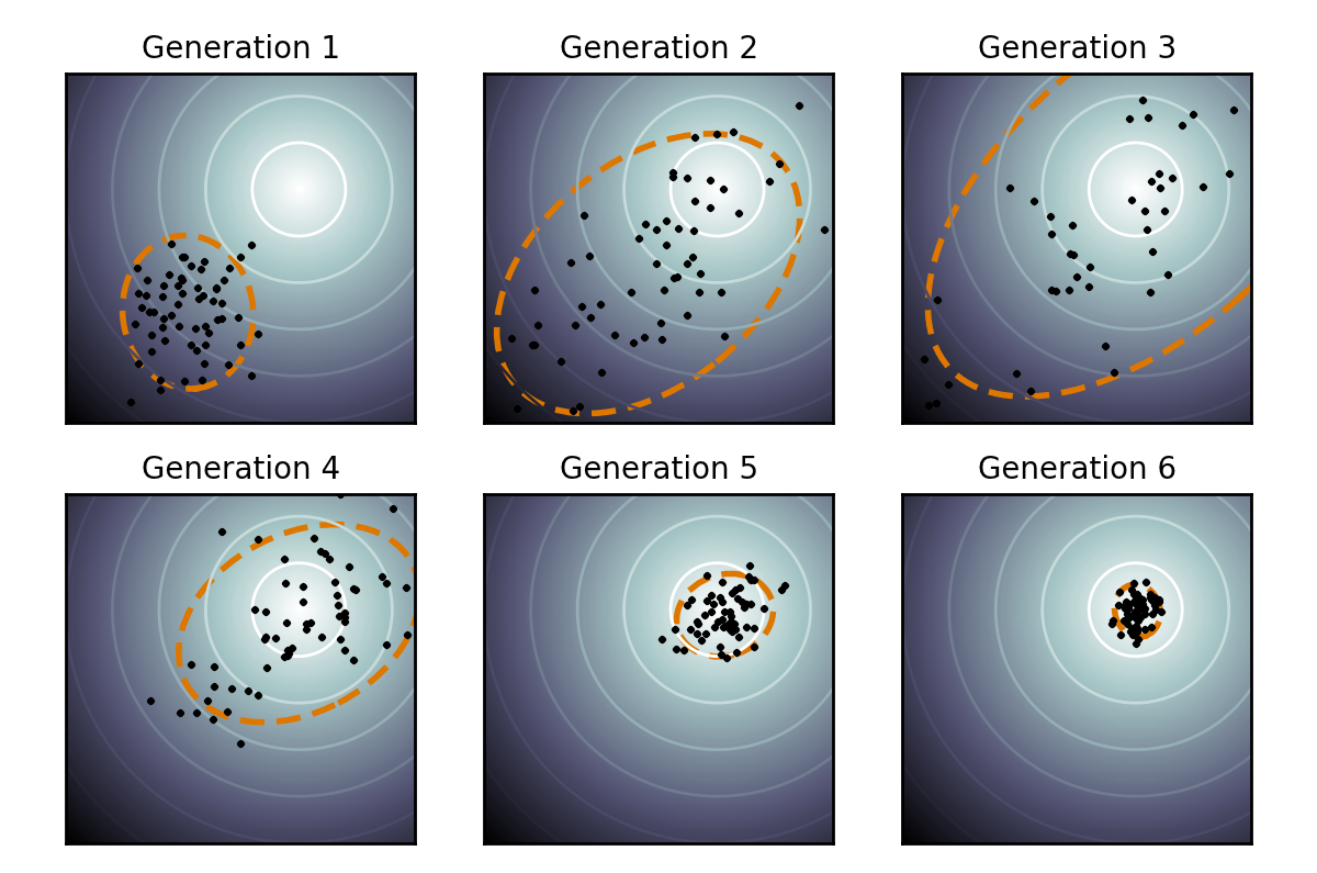
CMA-ES cost landscape example
For each generation, it performs three key steps:
- Sampling: It generates a new population of solutions from a Gaussian distribution defined by its mean (the current best guess), its step-size (sigma), and its covariance matrix (the shape and orientation of the distribution).
- Evaluation: It calculates the “fitness” or “cost” of each solution by running a simulation and seeing how well it performs.
- Update: It updates the distribution’s parameters (mean, step-size, and covariance) based on the ranking of the solutions. The mean is shifted towards the better-performing solutions, and the covariance matrix is adapted to better align with the directions of successful steps.
This process allows CMA-ES to efficiently explore the search space and converge on optimal solutions. The structure of our cost function is critical because it creates a “landscape” that CMA-ES can navigate effectively.
The Staged Cost Evaluation
A controller with random parameters is highly unlikely to produce a stable walking gait. Most initial values and hand-tuning will result in the model falling sooner or later. Thus, we provide a gradient of feedback that tells the optimizer how badly a solution failed.
To achieve this, our framework uses a three-stage cost evaluation system. The cost returned is designed to be orders of magnitude different at each stage, creating a clear path for the optimizer to follow.
Simulation Error (Cost ≈ 1.2E6)
This is the penalty for simulations that fail to complete. An early termination can be triggered by the following errors:
- Invalid physics states (e.g.,
NaNvalues). - No detected ground reaction forces (e.g., model not contacting the ground properly, or incorrect sensor placement)
- Invalid initial pose (e.g., model intersecting ground)
e.g. walk_cost.py
        Myo_env.reset(params)
        pose_valid = Myo_env.check_pose_validity()

        if not pose_valid:
            return 120 * 10000
Note: debug prints for this cost value can be found in reflex_interface.py.
If one of these errors is triggered at the start of optimization, it is unlikely to change. CMA-ES will (more often than not) terminate due to stagnation. However, it is possible for these cost values to occur within a population throughout optimization. CMA-ES will not terminate as long as 1.2E6 is not the best overall cost of an iteration.
Stage 1: Early Termination (Cost ≈ 9.8E4)
A cost of ≈ 9.8E4 represents a successful environment initialization and the standard initial CMA-output cost value if all is well when running an optimization without initial parameters. However, the model is still falling. This cost structure rewards controllers that can remain upright for longer, even if they don’t complete the full simulation.
def calculate_early_cost(cost_const: float, data_store: List[Dict], left_stance_foot: List[int], right_stance_foot: List[int], failure_mode: int = 99) -> float:
    """Calculate cost for early termination cases."""
    total_cost = (
        failure_mode * cost_const -
        (data_store[len(data_store)-1]['obj_func_out']['pelvis_dist'][0]) -
        (0.5 * (len(left_stance_foot) + len(right_stance_foot)))
    )
    return total_cost
Stage 2: Constraint Violation (Cost ≈ 1.0E4)
A simulation may run to completion but still not produce a desirable walking gait. This stage assigns a medium-tier penalty if the controller fails to meet additional constraints.
The primary constraints are:
- Minimum Strides: The model must complete a minimum number of successful strides (e.g., 5).
- Symmetry: The timing of left and right footfalls must be symmetric within a threshold.
- Velocity: The average velocity must be close to the target velocity.
- Pelvis Orientation: The pelvis must remain reasonably upright (for 3D models).
Values for these thresholds and targets are set through the config files and in train.py (Running_Optimizations).
If these constraints are not met, the cost is calculated as:
Example constraint penalties:
- Velocity penalty:
100 × velocity_cost × (velocity_cost > 0.01) - Symmetry penalty:
100 × sym_cost × (sym_cost > tgt_sym)
Stage 3: Final Performance Cost (Cost < 1.0E3)
If a controller produces a valid walk that passes all constraints, it is evaluated with a final performance cost. This final cost is a weighted sum of several metrics, determined by the chosen optimization type (e.g., -eff, -kine, -vel). Different final cost functions will produce different results.
This cost is on a much lower scale (typically in the hundreds, but varies by cost function), signaling to the optimizer that it has found a “good” region of the search space and should now focus on fine-tuning the performance.
Cost Components Explained
The final performance cost is assembled from various components, each quantifying a specific aspect of the gait.
Effort Cost (Cost of Transport)
Measures the metabolic energy efficiency of the gait. It is calculated as the sum of squared muscle activations over the evaluation period, normalized by the model’s mass and the distance traveled.
Kinematics Cost
Measures how closely the model’s joint angles match a set of reference kinematics. The controller’s gait cycle for each joint is interpolated to 100 points and compared to the reference data. The reference data provided is normalized joint angles for a single gait cycle.
The per-stride joint angles are interpolated to 100 points and compared to reference. The absolute error is averaged over the detected strides. The trunk term is computed separately and added with weight 1 in final costs that include kinematics.
Velocity Cost
Measures the difference between the average stride velocity and the target. The forward and lateral components are considered (on slopes, forward is computed in the x–z plane).
Ground Reaction Force (GRF) Cost
Penalizes GRF exceeding an upper threshold. We sum the exceedance of the total vertical GRF (left+right) over the evaluation window and normalize by duration.
Joint Limit Cost (Pain Cost)
Penalizes the controller for relying on joint-limit torques, which represent the passive ligaments and structures of the joints rather than active muscle control.
EMG Profile Cost
Similar to the kinematics cost, this measures the difference between the model’s muscle activation patterns and reference EMG data from human subjects.
Symmetry Cost
Computed at detected left/right stance events using Euclidean differences of knee and ankle positions relative to the pelvis, averaged over the requested number of strides.